Knight’s Tour Adjacency Matrix Visual
Self-Directed
R
Below you will find a Shiny App made for fun using concepts learned in Linear Algebra and Computational Linear Algebra, most notably graphs, adjacency matrices, matrix exponentiation, and Markov chains. All of the key concepts used to build the app are explained if you are interested in learning what is going on behind the scenes.
Shiny App
The Math Behind the App
Adjacency Matrices
An adjacency matrix is a type of matrix used to represent a mathematical graph, as pictured below:
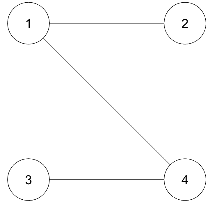
The matrix shows which vertices in a graph are adjacent to one another and which are not. It can be thought of as this: the rows are the starting points and the columns are the ending points. If you can get from a starting point to an ending point, then a 1 is placed, and otherwise it is 0.
\[ A = \begin{bmatrix} 0 & 1 & 0 & 1 \\ 1 & 0 & 0 & 1 \\ 0 & 0 & 0 & 1 \\ 1 & 1 & 1 & 0 \\ \end{bmatrix} \]
For example, in our graph, 2 and 4 are connected. If you look in the 2nd row (the starting place) and then at the 4th column (the ending place), you will see that there is a 1. Conversely, if you look at \(A_{2,3}\), you will see that it is 0, meaning 2 and 3 are unconnected, which can be confirmed by looking at the graph. These types of matrices are always square \(n \times n\) matrices because the same vertices are shown in both the rows and the columns. How this relates to a knight is as follows: if you imagine the 64 squares on a chessboard as vertices, we can graph the connecting vertices to show what the knight can reach in one move (later on, we will extend this to multiple moves, but we are not there yet).
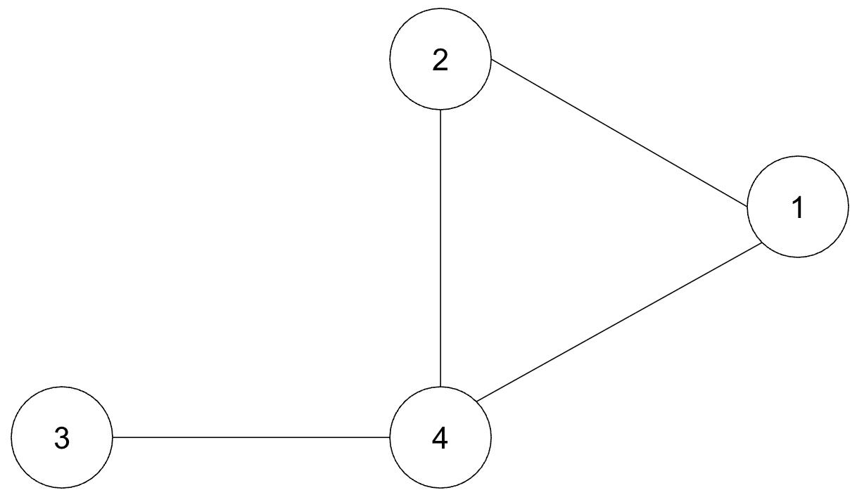
However, chess squares have fixed positions. In this graph, 1 could be placed to the right of 4 and it would not matter, as seen below.
Lattice Adjacency Matrices
We need to introduce a system of order to the graph to make it more of a rigid grid. This is precisely why using a Lattice graph is so helpful in this case. Lattice graphs offer distinct coordinates, or lattices, which line up exactly with what we want to do with the chess squares because each square is distinct and has 2-dimensional coordinates (i.e. the square (1, 2) has an x dimension and a y dimension).
\[ \begin{gather*} \begin{bmatrix} (1,1) & (1,2) & (1,3) \\ (2,1) & (2,2) & (2,3) \\ (3,1) & (3,2) & (3,3) \\ \end{bmatrix} \\ \text{Lattice Matrix} \end{gather*} \]
Just as we made an adjacency matrix from a normal graph, we can make a lattice adjacency matrix from a lattice graph. For our purposes, lattice matrices are just regular matrices, but each entry in the matrix represents a lattice point (i.e., \(A_{1,1}\) represents the lattice point (1,1)).
In order to make a lattice adjacency matrix given \(n \times n\) lattices, we will essentially construct an \(n^2 \times n^2\) matrix. This comes directly from what we did with the adjacency matrices; every single node was placed both horizontally and vertically in order to show every pair of connections between the nodes. In this case, since our grid has \(n \times n = n^2\) lattices, the matrix will be much larger. Essentially, what we are doing is making a long vector out of the lattice and then making that long vector 2D by taking the outer product of two long vectors.
\[ \begin{gather*} \begin{bmatrix} \textcolor{red}{1} & \textcolor{red}{2} & \textcolor{red}{3} \\ \textcolor{blue}{4} & \textcolor{blue}{5} & \textcolor{blue}{6} \\ \textcolor{green}{7} & \textcolor{green}{8} & \textcolor{green}{9} \\ \end{bmatrix} \longrightarrow \begin{bmatrix} \textcolor{red}{1} \\ \textcolor{red}{2} \\ \textcolor{red}{3} \\ \textcolor{blue}{4} \\ \textcolor{blue}{5} \\ \textcolor{blue}{6} \\ \textcolor{green}{7} \\ \textcolor{green}{8} \\ \textcolor{green}{9} \\ \end{bmatrix} \longrightarrow \begin{bmatrix} 1 \\ 2 \\ 3 \\ 4 \\ 5 \\ 6 \\ 7 \\ 8 \\ 9 \\ \end{bmatrix} \begin{bmatrix} 1 & 2 & 3 & 4 & 5 & 6 & 7 & 8 & 9 \end{bmatrix} \longrightarrow \begin{bmatrix} &1 & 2 & 3 & 4 & 5 & 6 & 7 & 8 & 9 \\ 1 \\ 2 \\ 3 \\ 4 \\ 5 \\ 6 \\ 7 \\ 8 \\ 9 \\ \end{bmatrix} \\ \space\space\text{Lattice}\space\space\space\space\space\space\space\text{Long Vector}\space\space\space\space\space\space\space\space\space\space\space\space\space\space\space\space\space\space\space\space\text{Outer Product}\space\space\space\space\space\space\space\space\space\space\space\space\space\space\space\space\space\space\space\space\space\space\space\space\space\space\space\space\space\space\space\space\space\space\space\space\space\space\space\space\space\space\space\text{2D Long Vector}\space\space\space\space\space\space\space\space\space\space\space\space\space\space \end{gather*} \]
Making the Lattice Adjacency Matrix
Now that the matrix is made, we can use the 2D to 1D conversion formula: \((\text{row} -1) \times \text{row length} + \text{column}\). This helps streamline the process of actually assigning what squares are adjacent to one another when a knight jumps. For every single cell, we can just calculate the knight moves with a helper function and then assign them a 1 or 0 if they are adjacent.
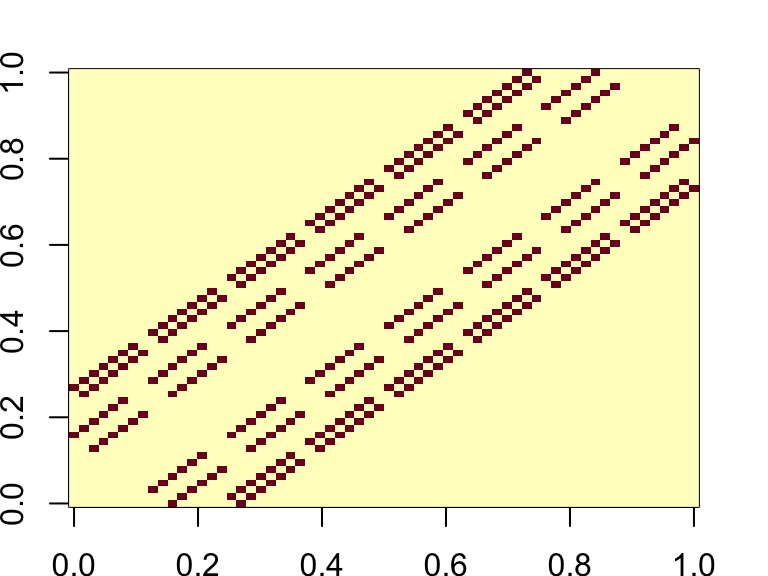
The end result looks like this:
Now, the reason why we wanted to go through all this trouble was because adjacency matrices are very useful for showing future movement from any starting point. This is done as easily as just exponentiating the adjacency matrix \(A\) to some degree \(n\). In doing so, from the basic properties of matrix multiplication, we can determine all of the possible paths of length \(n\) that start and end anywhere. For example, by taking the matrix \(A\) from before (representative of Graph 1), computing \(A^2\), and zooming in on the results for the paths that end at node 2 after 2 walks, we can see this clearly:
\[ \begin{equation*} \begin{gathered} A = \begin{bmatrix} 0 & 1 & 0 & 1 \\ 1 & 0 & 0 & 1 \\ 0 & 0 & 0 & 1 \\ 1 & 1 & 1 & 0 \\ \end{bmatrix} \\[1em] A \times A = \begin{bmatrix} \cdot & \color{red}{(0 \cdot 1) + (1 \cdot 0) + (0 \cdot 0) + (1 \cdot 1)} & \cdot & \cdot \\ \cdot & \color{red}{(1 \cdot 1) + (0 \cdot 0) + (0 \cdot 0) + (1 \cdot 1)} & \cdot & \cdot \\ \cdot & \color{red}{(0 \cdot 1) + (0 \cdot 0) + (0 \cdot 0) + (1 \cdot 1)} & \cdot & \cdot \\ \cdot & \color{red}{(1 \cdot 1) + (1 \cdot 0) + (1 \cdot 0) + (0 \cdot 1)} & \cdot & \cdot \\ \end{bmatrix} = \begin{bmatrix} \cdot & \color{red}{1} & \cdot & \cdot \\ \cdot & \color{red}{2} & \cdot & \cdot \\ \cdot & \color{red}{1} & \cdot & \cdot \\ \cdot & \color{red}{1} & \cdot & \cdot \\ \end{bmatrix} \\[1em] \begin{array}{c c l} \textbf{Start} & \textbf{Count} & \textbf{Explanation} \\ 1 & 1 & \text{1 path from node 1 of } \textcolor{red}{\text{length }\textbf{2}} \text{ to node 2} \\ 2 & 2 & \text{2 paths from node 2 of } \textcolor{blue}{\text{length }\textbf{2}} \text{ to node 2}\\ 3 & 1 & \text{1 path from node 3 of } \textcolor{green}{\text{length }\textbf{2}} \text{ to node 2}\\ 4 & 1 & \text{1 path from node 4 of } \textcolor{purple}{\text{length }\textbf{2}} \text{ to node 2}\\ \end{array} \end{gathered} \end{equation*} \]
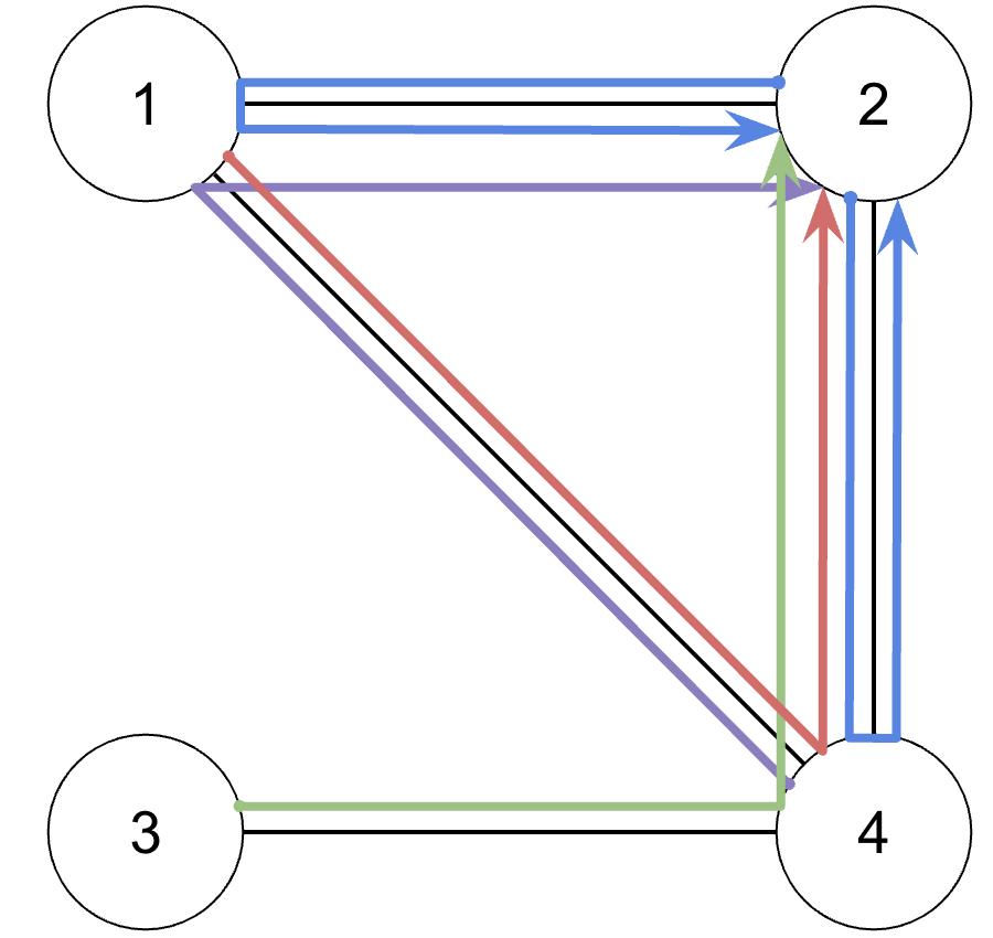
Here it can clearly be seen that, just as before, when we look at the column 2, we find all of the nodes that have a connection with node 2, but this time it is if they have a path of 2 walks (from raising \(A\) to \(n = 2\)). This allows for there to be more numbers than just 0 and 1 as it’s possible that nodes have 2 ways to get to node 2 in 2 moves, just like in the case of node 2.
And there is no limit on how high the exponent can go– meaning that if it weren’t for computation time or the bigger inhibitor of digit space, the shiny app can display thousands of moves into the future.
What It All Means
While this project may not be the most practical application, the patterns that emerge in the app highlight broadly useful concepts from linear algebra. If you interact with the app long enough, you will notice that certain squares — particularly the central squares — consistently have the highest count or probability of the knight landing on them. This behavior mirrors the idea of eigenvalues in a matrix, which predict long-term behavior: in this case, how the tiles’ ‘popularity’ evolves after multiple moves. Eigenvalues essentially tell us the dominant patterns of movement that emerge after many iterations, with higher eigenvalues corresponding to squares that are more likely to be landed on.
In some setups, there is a switch between light squares dominating or dark squares dominating depending on whether the exponent is odd or even. This is a result of the bipartite nature of the board: the board can be divided into two distinct sets of squares (light and dark), and squares within each set are not connected to others of the same set. This property is crucial because it suggests that the eigenvalues of the matrix governing the knight’s movement are symmetric around zero. Specifically, for matrices with this symmetry, we have \(\lambda \times m = -\lambda \times m\), which explains why odd and even powers of the matrix lead to such different behaviors. The switch between the odd and even powers of the matrix helps to explain the shifting dominance of the squares. When we raise the matrix to odd powers, the behavior tends to favor one set (either light or dark squares), while raising it to even powers leads to a more balanced or alternating pattern, as the symmetry of the eigenvalues becomes more apparent.
Adjacency matrices can be very powerful tools, helping with topics such as the spread of infectious disease, Google’s PageRank, and weather forecast.
References
Brualdi, Richard. “The Mutually Beneficial Relationship of Graphs and Matrices.” CBMS Regional Conference Series in Mathematics, vol. 115, no. 1, 6 July 2011, pp. 14–23, www.ams.org/bookstore/pspdf/cbms-115-prev.pdf, https://doi.org/10.1090/cbms/115. Accessed 9 Sept. 2025.